An effective approach to such an adaptive stopping criterion is to modify the
likelihood function of Eq. (3) so that it becomes flatter in the
vicinity of a good fit. The approach I have taken is to use a likelihood
function that is identical to Eq. (3) when the difference between the
blurred model and the data
is large compared with the noise, but that
is essentially constant when the difference is smaller than the noise.
There are two important advantages to using a modified form of the likelihood function to control noise amplification:
It is appropriate to prevent noise amplification by recognizing its effects in the data domain rather than by applying regularizing constraints on the restored image. Residuals that are smaller than one expects based on the known noise properties of the data should be avoided by using a likelihood function that does not reward overfitting the data. Of course, it may be necessary to use constraints on the model image in order to select one of the many possible restored images that fit the data adequately well, but in my opinion it is important to first establish better goodness-of-fit criteria so that the set of possible restored images is as small as possible before applying regularization to select one of those images. The work of Piña &Puetter (1992) on the Maximum Residual Likelihood criterion for data fitting is a notable attempt in this direction.
The damped R-L iteration starts from the likelihood function
where
and
is the ``damping function''. It is chosen to be a simple function that
is linearly proportional to
for
, is approximately constant for
, and has continuous first and second derivatives at
(this allows
acceleration techniques to be used to speed convergence of the method). The
constant
determines how suddenly the function
becomes flat for
.
For
,
and there is no flattening at all. The larger the value of
, the flatter is the function. The results reported in this paper use
, but the value of
has little effect on the results as long as it is
larger than a few.
is a slightly modified version of the
function of
Eq. (3). The constants and multiplicative factors are chosen so that
the expected value of
in the presence of Poisson noise is unity if the
threshold
. The threshold
then determines at what level the damping
turns on: if
the damping occurs at
, if
at
,
etc.
With this new likelihood function, we can follow the steps outlined above to derive the damped R-L iteration:
where
Note that in regions where the data and model do not agree, and so this iteration is exactly the same as the standard R-L iteration.
In regions where the data and model do agree, however, the second term gets
multiplied by a factor which is less than 1, and the ratio of the numerator and
denominator approaches unity. This has exactly the desired character: it damps
changes in the model in regions where the differences are small compared with
the noise.
Fig. 3 shows the results of applying the damped
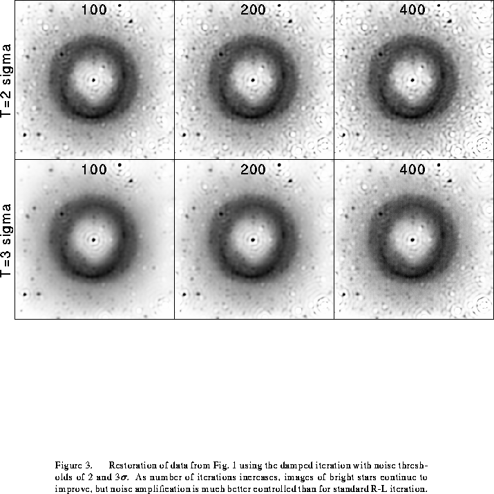
iteration to the planetary nebula data of Fig. 1. Note that the
noise amplification in the nebulosity has been greatly reduced, but that the
stars are still very sharp. Fig. 4 shows the result of applying
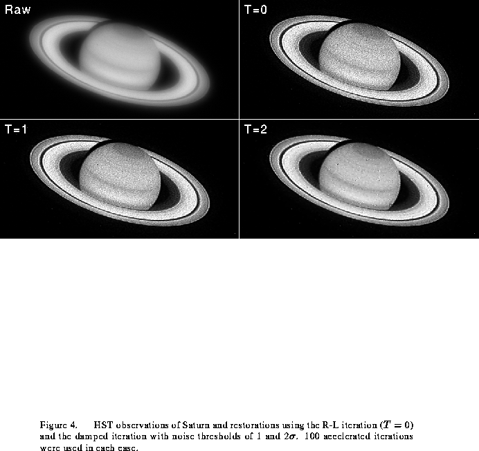
both the standard R-L method and the damped iteration to HST observations of
Saturn; again, the noise in the restored image is greatly reduced without
significantly blurring the sharp edges of the planet and its rings. This is
perhaps more easily seen in Fig. 5, which shows the brightness
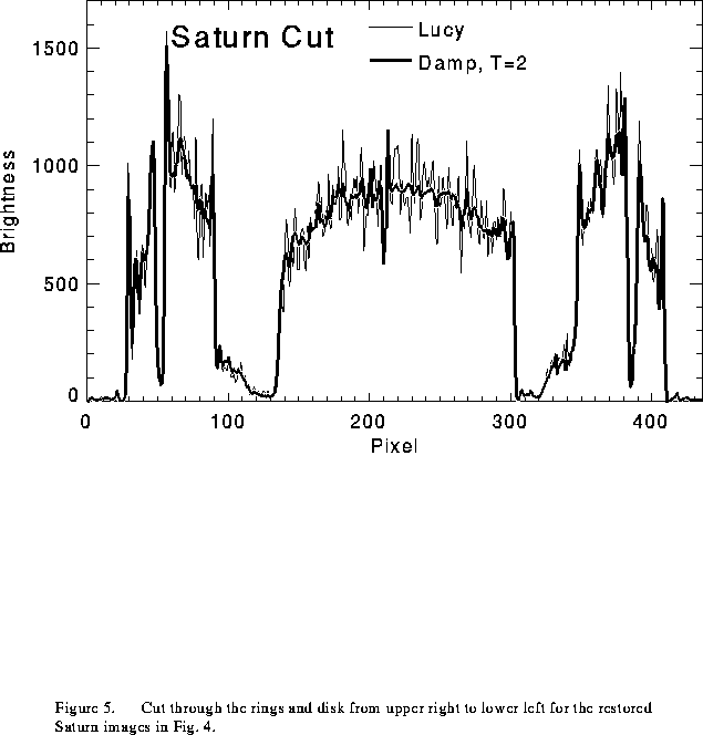
of the restored image along a cut through the planet and rings. Sharp features such as narrow gaps in the rings are essentially identical in the R-L and damped images, but the disk of the planet is much smoother in the damped image. Note that the mean brightness in the disk of the planet is the same in the damped and R-L images, indicating good photometric linearity.