Quick Start: Diving into data reduction

This is a quick tutorial to help new users get familiar with the GPI pipeline. More detailed documentation of the tools shown here can be found on subsequent pages.

Sample Data Reduction Tutorial

As an introduction to reducing data with the GPI Pipeline, a simple set of data is available on the Canadian Astronomy Data Center (CADC). If it is the first time you visit CADC, you will need to register. Once completed, go into the gpi directory and download the GettingStarted_tutorial_dataset folder. This contains a small set of data to give an overview of the different types of image and how to process them. All the files are raw data coming from the detector and we will reduce them one at a time.

Note

It is important that the user follow the tutorial in the displayed order. Skipping steps will result in reduction errors (missing calibrations etc).

The GPI Pipeline GUIs

It is assumed you have successfully launched the pipeline following the previous sections.(If not, see the GPI Data Pipeline Installation & Configuration manual.) Therefore, you should have the two IDL sessions opened with the GPI launcher GUI and the GPI DRP status console below. See Starting the GPI Data Pipeline and Starting the GPI Data Pipeline. The GPI pipeline console should indicate something like:

|    Now polling for DRF files in /Users/yourusername/somedirectory/GPI/queue/

The Launcher Window

The Launcher is a little menu window that acts as the starting point for launching other tools. In this getting started tutorial, we will mostly use GPItv and the Recipe Editor tools.

The Status Console

This lets you see the current execution status, view log messages, and control certain aspects of the pipeline. See Status Console for more details.

Contents of the Sample Dataset

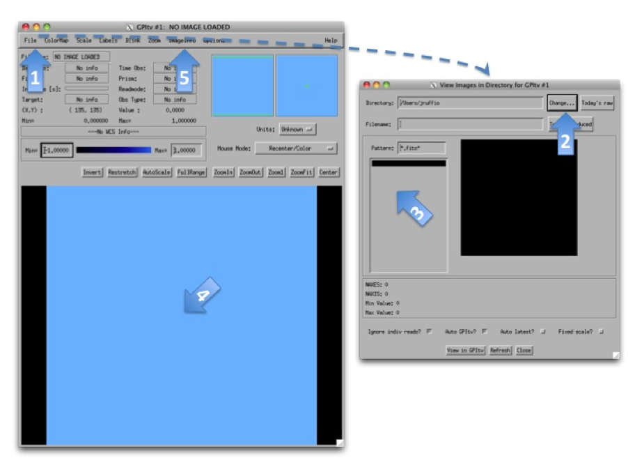
Before reducing any files, the best is probably to take a look at the raw data we have using GPItv. Click on the GPItv button on the GPI launcher to open it (See GPItv Viewer User’s Guide for more details):

1. Then File->Browse Files...,
2. In the new window push the button Change... and select a folder in the GettingStarted_tutorial_dataset.
3. The .fits files list should appear.
4. As you select one file or another, the GPItv window should refresh and plot the new image.
5. Use the GPItv menu File->View FITS headers... to get detailed information for each image.
6. Click on the image to center the view on a pixel. Adapt the zoom with the buttons.

Feel free to experiment with the GPItv GUI and try out different functions. Most concepts should be straightforward to anyone familiar with ds9 or especially atv.

Description and preview

• The two folders called darks_60s and darks_120s contain darks images with different integration times (respectively 58.19 and 119.29 seconds [1] ). An example of a raw dark image is shown below. We can see horizontal stripes caused by correlated noise introduced during the detector readout. They will be removed by the pipeline.

• The wavelength_cal folder contains Xenon arc lamp calibration data. An example image is shown below. These images are much more interesting because you can observe particular wavelength positions for the lenslets. These data are used to calibrate the wavelength solution for each of the different lenslets. Given the orientations of IFS spectral prism and detector, shorter wavelengths are closer to the top of the detector for each lenslet (i.e. have higher Y pixel values) while longer wavelengths extend down toward the bottom.

• The onsky_data directory contains a raw coronagraphic image that we wish to reduce (the central section is shown below). Each microspectrum consists of the light from a 14.3 by 14.3 milli-arcsecond section of the field of view. The pipeline will extract each spectrum and create a 3 dimensional data cube, where each 2-dimensional slice of the cube corresponds to a given wavelength.

• The files_to_go_into_calibrations_directory directory contains files that must be copied over into your calibrations directory, as defined by the environment variable GPI_DRP_CALIBRATIONS_DIR that was declared upon the pipeline configuration. After copying these files into this directory, the user must click on Rescan Calib. DB button, located in the bottom left hand corner of the GPI DRP Status Console. Files in this directory include a bad pixel map, a microphonics model, and a flexure shifts lookup table.

Footnotes

[1]

The reason for these odd exposure times is that GPI IFS exposures are quantized in units of the readout time for the detector, 1.45479 seconds. Because of this quantization, in practice one typically just rounds the durations, so these would be e.g. “60” and “120” second exposures - there’s no need to carry around all the significant figures.

General reduction method

Let’s first give the general method to reduce any file. This will then be applied in the next sections for different particular cases. Only the selected items in the different option lists will change.

Press the Recipe Editor button in the GPI Launcher window and the window below will open.

Note

The principle of the pipeline is based on recipes to reduce files. A recipe includes a list of input files (the ingredients) and a list of primitives to be applied on those files (the actions). Each primitive is an elementary algorithm to be applied on files listed in the recipe. The action can be anything, for instance subtract dark frame or build data cube. There are two kinds of primitives: ones that should be applied on each file and ones that are applied on all files together. For instance, Subtract Dark acts on one file at a time, while Combine 2D images will merge all the files from the list resulting in a single output file. The special primitive Accumulate Images divides the two categories of primitives. All the primitives before are applied to each file, then Accumulate Images gathers up the results, and any primitives after are applied to the entire set.

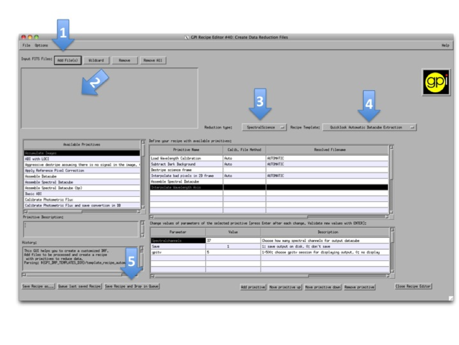
The numbers of each of the following steps match with the screenshot above.

1. Press the upper-left button Add File(s) and select the files to reduce.
2. The selected files should appear just below.
3. Select the reduction type in the menu.
4. Select a Recipe Template. You may want to change the recipe if it doesn’t match exactly to your expectation. It is possible to add, move and remove any primitive and also to change various input parameters that adjust algorithm details.
5. Press Save Recipe and drop in queue button. This will generate the recipe based on the selected files and the list of primitives. The recipe is automatically saved in the queue directory, meaning that it will be read as soon as the pipeline is idle. The reduction might take a while depending on the computer.

In the following, these steps will be repeated several times with specific indications.

Note

For every reduction, a gpitv window will open with the result of the reduction and the file will be saved in the reduction folder defined when installing the pipeline. If you don’t want to plot or to save the results, you can change the parameters Save and gpitv of the primitives. To change parameters, select the primitive in the upper right table. Then, its parameters will appear in the bottom right table. Select the value of the parameter and type what ever is asked. Finally, press enter to validate the input.

Note

The recipe templates often only work in a particular context, meaning that if you try to apply one of them to a random file it probably won’t work and the pipeline may crash. It is because the primitives are yet not very robust and they need more or less exactly the inputs they were designed for.

Reduce your calibration and Science files

Darks

The dark calibration files for a given integration time can be combined using these amendments to the Recipe Editor usage steps above:

• For step 1) Select the 60s darks: S20131208S0016(-20).fits.
• For step 3) Choose the Calibration Reduction type.
• For step 4) Choose the Dark Recipe template.

The 60s darks correspond to the science data and will be used in the following section.

The selected primitives are then:

• Aggressive destripe (assuming there is no signal in the image): This should remove the apparent lines in the image that come from the readout of the pixels by the detector.
• Accumulate Image: Gather all the images of the recipe. It indicates that the subsequent primitives will apply to all images.
• Combine 2D dark images: Merge all the images with the same integration time using the median.

The GPI DRP Status Console will display a progress bar and log messages while reducing the files.

When reducing calibration files the result is automatically saved in the Calibrations folder. The path to this folder was defined when installing the pipeline and should normally be in the reduced folder (See Configuring the Pipeline $GPI_REDUCED_DATA/calibrations).

The pipeline will look for calibration files automatically by reading the text file GPI_Calibs_DB.txt in the calibration folder (see The Calibration Database). There is a button at the bottom of the GPI DRP Status Console called Rescan Calib. DB to create or refresh this text file.

Use the button Remove All to remove all the selected files then Redo this with the 120s integration times which corresponds to S20131208S0021(-22).fits. This newly created dark frame will be used to reduce the wavelength calibrations in the next section.

Wavelength solution

Like the dark frames, the wavelength solution calibration files can be created using the Recipe Editor reduction steps with the following additions:

• For step 1) Select Xe-arc lamp files: S20131208S0149(-151).fits.
• For step 3) Keep selected the Calibration reduction type.
• For step 4) Choose the Wavelength Solution Recipe template.

Note

If you did not correctly copy in the files from the files_to_go_into_calibrations_directory then you will get warnings but it should work anyway. How to create such files is described in the Step-by-Step reduction documentation

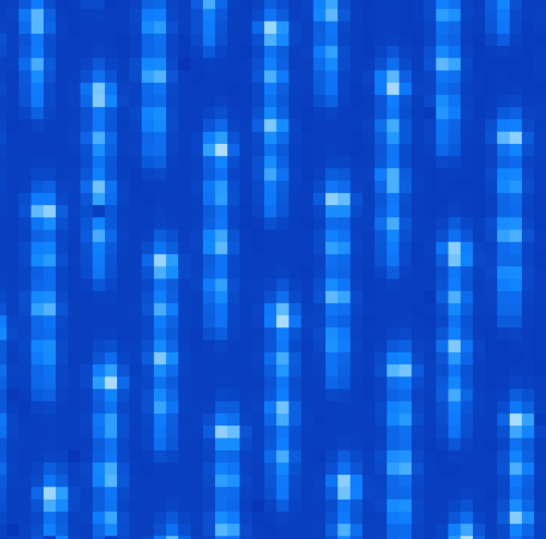
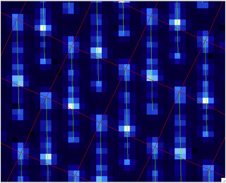
A sample of the 2D image with the computed calibration is given below. The green lines are the locations of the individual lenslet spectra. The coordinates of the lenslets are stored in a .fits file cube in the calibrations folder. Use GPItv to take a look to the result.

Reducing your science data

The following is an example of how to reduce science data. - For step 1) Select your science data S20131210S0025.fits. - For step 3) Select the SpectralScience reduction type. - For step 4) Choose the Quicklook Automatic Datacube Extraction Recipe template.

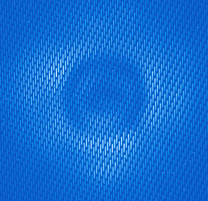
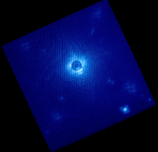
All the calibration files are automatically found and the result is a final data cube. The result should be plotted in GPItv at the end of the reduction. Feel free to look at the different wavelengths by changing the selected slice. Note that this example does not account for the flexure offsets between the wavelength calibration derived above, and the current spectral positions, therefore the reduced cube will be rather ugly and have a large Moire pattern in the data.

In order to correct for this, we must account for the offsets. If one opens the raw image in GPItv, then overplots the wavelength soluution (Labels -> Get Wavecal from DB, then Labels -> Plot Wavecal Grid -> Draw Grid), one will see the large offets (shown below).

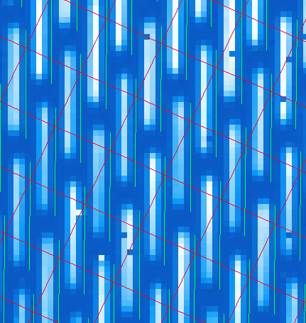
As a rough approximation, one can input offsets in GPItv (in the plot wavecal grid) until the overlap looks correct (note that old drawings of the wavecal can be erased by Labels -> Erase All). An (X,Y) shift of (-2,1) is a reasonably good guess. The user can then input these offsets into the ‘Update Spot Shifts for Flexure’ primitive. To do this:

1. Click on the Update Spot Shifts for Flexure primitive in the recipe window.
2. Change the method keyword to, “Manual” in the primitive parameters window (just below the recipe window)
3. Change the manual_dx and manual_dy keywords to the desired values.
4. Re-run the reduction (Save Recipe and Queue)

Because a snapshot of the Argon arclamp was taken at the same telescope position, we can use this to determine the needed offsets in a much more robust fashion.

• For step 1) Select the Ar-arc snapshot taken with the data: S20131210S0055.fits.
• For step 3) Keep selected the Calibration reduction type.
• For step 4) Choose the Quick Wavelength Solution Recipe template.

This primitive will use every 20th lenslet in the frame to calculate the net shift from the desired wavelength calibration. One must be careful to ensure the proper wavelength calibration is grabbed from the database (check the output in the pipeline xterm). If the wrong one is selected, then you can manually choose the correct one (S20131210S0055_H_wavecal.fits) using the Choose Calibration File button. A new wavecal (S20131210S0055_H_wavecal.fits) will then be added to the database, which is merely the old wavecal with new x-y spectral positions.

If you now repeat the reduction of the science data from above, the new wavecal will be captured and the datacube will appear as follows. Remember to set the “Update spots shifts for Flexure” correction to ‘none’

Enjoy the first of many data cubes!