[Top] [Prev] [Next] [Bottom]
30.6 Assessing FOS Science Observations
After checking the target acquisition you may want to know whether the requested science integration time requirements were actually fulfilled. The exposure logsheet (see exposure number 4 in Figure 30.11) gives only a first estimate as requested exposure times were often modified by up to 20% to facilitate efficient orbit-packing. The actual on-source integration times are stored in the headers of the science data (e.g., the .c1h and .c0h files), in the header keyword EXPTIME. The Exposure Summary section of the FOS paper products Observation Summary page also provides this information. For example, logsheet exposure 4 in Figure 30.11 requested an exposure time of 33 minutes, but reference to Figure 30.10 shows that the actual integration time with the G270H grating was shortened to 26 minutes in order to fill the orbit up to occultation.
Alternatively, if an exposure should be much shorter than was planned, check whether the observation was interrupted by an earth occultation. In this case, the integration will have been resumed as a separate exposure with a new rootname after re-acquisition of the guide stars following the occultation. In the example of logsheet exposure 6 in Figure 30.11 a 100 minute exposure with grating G190H was requested. As shown in Figure 30.10 the initial G190H exposure could last only 17 minutes prior to occultation. A new G190H 48 minute exposure complete with separate rootname and data products entirely filled the next orbit and yet a third separate exposure of 35 minute duration in the orbit following rounded out the complete 100 minute exposure time requested. (If the proposer had used the appropriate RPS2 command, the last orbit could have been completely filled, but it was not in this case.) Since the three exposures were obtained in different orbits on different guide star re-acquisitions, it is important to check that no pointing or guiding anomalies have occurred and that all have produced comparable photometric results.
 FOS exposures were not interruptible. Once data-taking stopped for occultation or
SAA passage, the exposure was terminated. Upon target re-acquisition a new
exposure began with a new observation rootname and resulted in a completely
new set of science data products. Prior to co-adding such exposure segments they
should be carefully compared to look for photometric or other differences that
could be associated with pointing or guiding.
FOS exposures were not interruptible. Once data-taking stopped for occultation or
SAA passage, the exposure was terminated. Upon target re-acquisition a new
exposure began with a new observation rootname and resulted in a completely
new set of science data products. Prior to co-adding such exposure segments they
should be carefully compared to look for photometric or other differences that
could be associated with pointing or guiding.
In the following sections we describe the details of each spectroscopic mode of FOS scientific data taking, namely ACCUM, RAPID, POLARIMETRY, PERIOD, and dispersed-light IMAGE. We describe the characteristics and structure of the mode-specific paper products and the electronic science data products. We will also provide guidelines concerning the analysis of the scientific data quality based upon evaluation of both the paper and electronic products.
The FOS paper products are useful for judging the quality of the spectra, including the quality of the calibration, the existence of artifacts, and the validity of specific features. Nonetheless, you may need additional detailed information on the single steps of the data calibration and on the characteristics of the instrument. Chapter 31 describes the pipeline calibration steps and how to recalibrate the data, which is always necessary. Chapter 32 delves into more detailed data analysis considerations, specifically error sources and attendant limiting accuracies for each of the major types of instrumental calibration.
The mode in which a given dataset was taken is identified in the data headers by the keywords OPMODE and GRNDMODE. The OPMODE (.shh) and GRNDMODE (.d0h, .c1h) keyword values are listed at the beginning of the output data products section in the following discussions of each of the individual science data-taking modes.
30.6.1 Spectrophotometry Mode (ACCUM)
Understanding ACCUM
ACCUM was the most commonly used FOS spectroscopic mode. ACCUM mode spectra with a total exposure time lasting more than a few minutes were read out at regular, equally sized, intervals to the ground or to the onboard tape recorders. The frequent readouts protected against catastrophic data loss. Since the data were read out at regular intervals, all observations longer than a few minutes (the time between readouts was usually about two minutes for FOS/RD and usually about four minutes for FOS/BL) were time resolved. The first readout was stored as group one, the next readout was added (accumulated) to the previous readout and the sum was stored as group two, and so on. The last group contains the spectrum from the full exposure time of the observation. The number of groups per observation depended on the length of the exposure and the detector used. Remember that for paired apertures and STEP-PATT not SINGLE, half of the specified exposure time was spent in each aperture with the data accumulated in alternating intervals of approximately 10 seconds.
Paper Products: ACCUM
ACCUM mode paper products produce three pages of mode-specific diagnostic plots. These are the flux vs. wavelength and log flux vs. wavelength page for the last group which contains the full exposure (see Figure 30.5), the corrected counts vs wavelength page for the last group (see Figure 30.6); and the group-by-group total counts plot (Figure 30.7). The last plot is particularly useful for assessing photometric repeatability and in revealing potential problems related to guiding, breathing, background, and intermittent noisy diodes. Please see additional notes in analysis section below concerning assessment of background count levels.
Output Data Products: ACCUM
Spectrophotometry mode is identified by an OPMODE keyword value of ACCUM and a GRNDMODE keyword value of SPECTROSCOPY. For the standard ACCUM mode, the default value of NXSTEPS was 4 and OVERSCAN was 5. ACCUM mode data files for SINGLE aperture exposures contain GCOUNT groups of 2064 pixels each. The .d0* and .c4* files of OBJ-OBJ or OBJ-SKY paired aperture observation data products may be longer as discussed in "Paired-Aperture File Structures" on page 30-6.
Analysis: ACCUM
In standard FOS ACCUM mode spectra the last group contains the accumulated total integration on the target. The paper products calibrated spectrum can be evaluated to check whether the flux level is roughly like that expected. (Alternatively, the IRAF/STSDAS task fwplot can also be used to perform this check.) If more than one detector readout occurred (i.e., the exposure was longer than two minutes for FOS/RD or four minutes for FOS/BL), use the paper products group counts plot to evaluate the overall photometric quality and repeatability of the measures. This plot can reveal the influence of poor guiding, breathing, re-centering events, and intermittent noisy diodes on individual groups that would normally not be expected from inspection of the last data group alone.
The background count rate is given in the Exposure Summary section and will be displayed in the paper product corrected count rate plot if it is on-scale. Although a model prediction of the background (and, for several dispersers, an approximation to the scattered light) has been removed from the quantities plotted in the paper products, it is useful to note that a 120 second total duration (30 seconds per pixel) standard FOS/RD ACCUM with 2064 pixels had a typical background component of 600-1200 dark counts per group. Similarly, a typical 240 second FOS/BL ACCUM exposure produced 900-1800 dark counts per group. It is often useful to compare this signal with the background-corrected quantity provided in the group counts plot. Extraction of individual group spectra can be accomplished with task deaccum (see "deaccum" on page 33-9).
If the spectrum was split up into two or more parts, for example because it was observed in more than one orbit due to occultations, you can obtain the sum of all integrations by adding up, with appropriate weighting, the last groups of all .c1 spectra of your target taken with the same instrument configuration (combination of detector, aperture, and disperser).
 For all but edge-pixels, the exposure time per pixel is not EXPTIME, but rather
EXPTIME/NXSTEPS. Pipeline calfos processing correctly manages the exposure
time for all pixels and populates the statistical error arrays according to actual
detected count levels for all pixels.
For all but edge-pixels, the exposure time per pixel is not EXPTIME, but rather
EXPTIME/NXSTEPS. Pipeline calfos processing correctly manages the exposure
time for all pixels and populates the statistical error arrays according to actual
detected count levels for all pixels.
30.6.2 Rapid Readout Mode (RAPID)
Understanding RAPID
For many astronomical targets where rapid variability in flux was suspected, but the precise period was unknown, or the expected variation was aperiodic, PERIOD mode of data acquisition was unsuitable because the bin folding period must be specified. In such cases the RAPID readout mode was used. RAPID mode was also used in cases where very strong signal would overflow the 16-bit FOS accumulators in the default ACCUM readout times (e.g., bright emission line sources). In this mode, the data were acquired using the normal substepping and overscanning techniques. The spectra were read out at intervals (chosen by the observer according to the scientific goals) that were much shorter than the normal four minute (FOS/BL) or two minute (FOS/RD) segments. Each readout was stored in the raw data file as a group. The number of groups in a RAPID mode observation .d0h file was equal to the number of individual readouts. For paired apertures and STEP-PATT not SINGLE, half of the specified exposure time was spent in each aperture with the data accumulated in alternating intervals of approximately 10 seconds or (readout time divided by 2), whichever was smaller.
Paper Products: RAPID
RAPID mode paper products produce three pages of mode-specific diagnostic plots. These are the flux vs. wavelength and log flux vs. wavelength page for the first group of the time-series (see Figure 30.5), the corrected counts vs wavelength page for the first group (see Figure 30.6); and the group-by-group total counts plot (Figure 30.7). As with ACCUM mode, the last plot is particularly useful for assessing photometric repeatability and in revealing potential problems related to guiding, breathing, background, and intermittent noisy diodes. Further, since the group counts plot is essentially a count rate light curve, it provides a quick look at a science objective of many RAPID readout programs. Please see additional notes in analysis section below concerning assessment of background count levels.
Output Data Products: RAPID
Rapid readout mode is identified by the keyword values OPMODE=RAPID and GRNDMODE=RAPID READOUT. There are GCOUNT groups of individual readouts. As with ACCUM mode, the default value of NXSTEPS is 4 and OVERSCAN is 5 and default spectrum length is 2064 pixels, however NXSTEPS was often modified by the user. The .d0* and .c4* files of OBJ-OBJ or OBJ-SKY paired aperture observation data products may be longer as discussed in "Paired-Aperture File Structures" on page 30-6 Additionally, the user could restrict the measured wavelength range, which produced a smaller number of pixels to be read out, and which dould, in certain circumstances, preclude scattered light correction.
The .c3h (special mode processing output - see next chapter) file contains two data groups. The number of pixels in each group is equal to the number of readouts (groups) in the original data. Group 1 of the .c3h file contains the summed flux values where the value of each pixel is the sum of all pixels from an original readout (i.e., pixel 1 contains the sum of all pixel values from readout 1, pixel 2 is the sum of all pixels from readout 2, etc. This is similar to, effectively a flux-calibrated version of, the information plotted in the paper products group counts display). Group 2 contains the sum of the corresponding statistical error values (in quadrature). The .c3h files effectively provide the light curve of the target for the length of the observation. See "Details of the FOS Pipeline Process" on page 31-13 for more details on special mode processing.
Analysis: RAPID
The IRAF/STSDAS task to combine groups in a RAPID mode dataset is rcombine (see Chapter 3).
Often RAPID mode observations were taken with NSXTEPS values other than four. The standard calibration software routinely handles these cases without special user intervention.
A few programs used OVERSCAN=1 to facilitate extremely fast readout. OVERSCAN=1 data are not calibrated by routine operation of calfos as all FOS reference files are based upon OVERSCAN=5 calibration observations. As an approximation in these cases, the first 2048 pixels of STScI reference files can be resampled for the appropriate NXSTEPS and, after editing the OVERSCAN value in the header, used with calfos. Archive researchers should keep in mind that these OVERSCAN=1 observations were not designed with the intention of producing accurate absolute photometry.
Many FOS/BL programs included RAPID mode time-series with the G160L grating. In addition to the ultraviolet spectrum, the zeroth order signal was also recorded. Therefore, white-light curves were often recorded in concert with the ultraviolet observations. Careful assessment of the count levels in the zeroth order spike should be made before attempting quantitative analysis as this very strong signal often produced accumulator wraparound (overflow) even in the relatively short readout times common in RAPID mode programs.
The background count rate is given on the Exposure Summary page and will be displayed in the paper product corrected count rate plot if it is on-scale. Although a model prediction of the background (and, for several dispersers, an approximation to the scattered light) has been removed from the quantities plotted in the paper products, it is useful to note and compare these quantities with the detected count rates as shown in the corrected count vs wavelength plot. A similar comparison with the group count plot levels can be made in which the average background count level can be estimated as (5 x readout time)
The RAPID mode readout time interval (logsheet entry READ-TIME) was not always constant in actual practice due to the internal operation of the FOS. Determination of the precise start and stop times of the individual readouts in many RAPID mode exposures requires special processing of engineering telemetry not normally available to the end user. If you need absolute or relative timing more precise than 0.125 sec, then you should contact help@stsci.edu for special support. Additional information on RAPID mode timing is found in "RAPID Mode Observation Timing Uncertainties" on page 33-5, as well as in the FOS Instrument Handbook, and in FOS ISR 154.
30.6.3 Spectropolarimetry Mode
Understanding SPECTROPOLARIMETRY
The polarimetry data consist of a number of exposures (POLSCAN=16, 8, or 4) with the waveplate set at different angles and taken consecutively (within one orbit). The Wollaston prism split the light beam into two spectra corresponding to the orthogonal directions of polarization. Hence, each exposure consists of the two orthogonal spectra obtained with a single waveplate angle. These spectra were deflected alternately onto the diode array, recorded as two pass directions, and stored as a single group in the raw data file. The first spectrum in the data group corresponds to the first pass direction (ordinary ray), the second to the second pass direction (extraordinary ray).
Paper Products: SPECTROPOLARIMETRY
There are no SPECTROPOLARIMETRY-specific paper product displays. The standard exposure summary, spacecraft performance, jitter ball, and calibration status pages are produced.
Output Data Products: SPECTROPOLARIMETRY
Spectropolarimetry mode1 is identified by an OPMODE value of ACCUM and a GRNDMODE value of SPECTROPOLARIMETRY.
The number of groups in the raw data file is equal to NREAD x POLSCAN. Thus, normally (for NREAD=1) there will be as many groups in the raw data file as the number of waveplate positions used in the observation. The number of POLSCAN positions (and therefore the total number of groups in the raw data file) may be 4, 8, or 16 depending on the number of polscans requested.
The group contents of the raw (.d0h) data file are shown in Table 30.8. Note that the number of pixels in each group is twice the number of pixels in a single spectrum as there are two spectra appended together, one for each pass direction. The number of pixels in the spectrum depends on the values of NXSTEPS and OVERSCAN used.
Group Contents of Raw -Polarimetry Science Data Files
The organization of calibrated polarimetry data files differs from the raw data files and calibrated data taken in other observing modes in that the two pass direction spectra from each readout are stored in separate data groups instead of being concatenated within one group. The calibrated fluxes, the corresponding statistical errors, and the data quality are stored in 2 x POLSCAN number of groups, similar to the wavelengths. Note that for polarimetry data the statistical errors cannot be combined simply. The errors in the Stokes parameters are calculated separately by the data reduction pipeline. The polarimetry-specific data are stored once again as groups in a separate file.2
The .c0h file is a dataset with 2 x POLSCAN groups with wavelengths for both pass directions through the Wollaston prism and each POLSCAN position. Note that the wavelengths for the different POLSCAN positions should be identical, but the wavelengths are offset between the two pass directions by a constant amount.
The .c1h file is a dataset with 2 x POLSCAN groups containing calibrated flux for both pass directions and each POLSCAN position. The calibrated fluxes are stored in exactly the same way as the wavelengths. Note that unlike calibrated flux data for non-polarimetric observations, the first group will not represent the absolute flux for the source, but only half, since the light was split into two spectra by the polarizer. Representative fluxes are formed by averaging the fluxes from the complete set of POLSCAN positions for each pass direction separately, and then summing the two. Since there is a wavelength shift between the spectra from the two pass directions, to combine the two mean spectra from both pass directions one spectrum must be shifted in wavelength to match the other. Pass direction 2 is shifted onto pass direction 1. In the summed spectrum, any pixel that has contributions from only one pass direction is set to zero. The total flux (Stokes I) is computed by the special mode processing phase of calfos and is stored in the .c3h dataset (see below) and so is more conveniently obtained from there.
The .c2h file is a dataset with 2 x POLSCAN groups with the statistical error of the calibrated flux for both pass directions and each POLSCAN position. The flux errors are stored in exactly the same way as the wavelengths and fluxes. As for the calibrated flux dataset, this dataset differs from the statistical errors for non-polarimetric data and the errors cannot be simply combined. We suggest that the error on the Stokes I parameter computed by the polarimetry processing be used as the total flux error.
The .cqh file is a dataset with 2 x POLSCAN groups with the data quality values for the calibrated fluxes. The organization is exactly the same as that of the calibrated fluxes dataset. The group organization of the .c0h, .c1h, .c2h, and .cqh files is shown in Table 30.9.
Group Organization of the Calibrated .c0h, .c1h, .c2h, and .cqh Files
Group
|
Contents Depending on Calibration File
|
|---|
|
1
|
Polscan 1, Pass direction 1: wavelength, flux, error or data quality
|
|
2
|
Polscan 1, Pass direction 2: wavelength, flux, error or data quality
|
|
3
|
Polscan 2, Pass direction 1: wavelength, flux, error or data quality
|
|
4
|
Polscan 2, Pass direction 2: wavelength, flux, error or data quality
|
|
...
|
...
|
|
31
|
Polscan 16, Pass direction 1: wavelength, flux, error or data quality
|
|
32
|
Polscan 16, Pass direction 2: wavelength, flux, error or data quality
|
The .c3h file is a dataset with 56 groups containing the reduced polarimetry data. The dataset is organized into four sets of 14 groups, where groups 1 through 14 contain the Stokes parameter and polarimetry data for pass direction 1, groups 15 through 28 for pass direction 2, groups 29 through 42 contain the merged data from both pass directions 1 and 2, and groups 43 through 56 contain the merged data corrected for interference and instrument orientation. The organization of the .c3h file is shown in Table 30.10.
Note that the wavelengths corresponding to the first set of 14 groups are given by the wavelength array for the first pass direction (i.e., group 1 of the .c0h file), while for the second set of 14 groups (groups 15 through 28) the corresponding wavelengths are given by the wavelength array for the second pass direction (i.e., group 2 of the .c0h file). For the merged data in the third and fourth sets of 14 groups (groups 29 through 56), the corresponding wavelengths are given by the first pass direction.
Analysis: SPECTROPOLARIMETRY
All polarimetric observations should be recalibrated. The polarimetric calibration portions of calfos will soon include special corrections to remove the influence of the COSTAR optics on polarimetric measures.
30.6.4 Time-Resolved Spectrophotometry Mode (PERIOD)
Understanding PERIOD
This mode was designed for objects with known periodicity in the 50 msec to 100 sec range. To maintain the phase information of these observations, the known period (CYCLE-TIME) of the object was divided into bins or slices, where each bin had a duration time = period/BINS. The spectra acquired in this mode were stored in the different bins which correspond to a given phase of the period. The information obtained in each period was added to the pattern so that the phase information was maintained (so long as the period was known accurately).
 Relativistic aberration is important for short periods and long observations. However, there is no correction for light travel time across the orbit.
Paper Products: PERIOD
There are no PERIOD-specific paper product displays. The standard exposure summary, spacecraft performance, jitter ball, and calibration status pages are produced.
Output Data Products: PERIOD
Time-resolved spectrophotometry mode is identified by the keyword values OPMODE=PERIOD and GRNDMODE=TIME RESOLVED.
The raw (.d0h) data file for time-resolved mode contains a single data group that is made up of all the individual spectral slices (or bins) stored sequentially. For example, if an observation used 374 detector channels, with NXSTEPS=1, OVERSCAN=5, and SLICES=32, the .d0h file would contain one data group having a total length of:
(374 + (5 - 1)) x 1 x 32 = 12096 pixels
The calibrated flux, wavelength, error, and data quality files will have the data from the individual slices (bins) broken out into separate groups. For the example above, the .c0h, .c1h, .c2h, and .cqh files would have 32 groups of 378 pixels.
The .c3h file is organized as follows. Groups 1 and 2 contain the average flux and average errors, respectively, of all the individual calibrated spectra. Following these, there are pairs of groups where the first group in each pair contains the difference between an individual flux spectrum and the average, and the second group in each pair contains the sum of the errors for the individual spectrum and the average. See "Special Mode Processing (MOD_CORR)" on page 31-23 for details on how the average and difference spectra are generated. For example, if the observation consisted of 32 slices, the structure of the .c3h file would be that shown in Table 30.11.
Group Structure of PERIOD Mode .c3h File with 32 Slices
Analysis: PERIOD
Only two scientific programs employed PERIOD mode. Due to implementation problems and errors, no PERIOD mode observations were completely successful. Successful tests were performed during Science Verification.
30.6.5 Image Mode Spectra (IMAGE)
Understanding IMAGE Spectra
FOS IMAGE mode observations imply mapping of more than one position in the aperture by the diode array. If a disperser was chosen as the spectral element, then spectra at YSTEPS y-positions, symmetrically spaced about the default aperture center Y-base were obtained. The specified exposure time was equally divided among the YSTEPS individual spectra, and was obtained in a continuing revolving series of approximately 10 second integrations at each individual Y-position until an exposure of EXPTIME was accumulated. Intermediate ACCUM-like readouts could occur. Although nearly all IMAGE mode FOS spectra were obtained for flux and flatfield calibration purposes, some measures of this type were used for the purpose of interactively acquiring moving targets with absorption lines at known wavelengths.
Paper Products: IMAGE Spectra
Figure 30.15 below shows an example of the one page of mode-specific FOS paper products for IMAGE mode spectra. Flux and wavelength calibrations are not routinely applied to IMAGE mode spectra as these calibrations are normally for the central y-levels of an aperture whereas an IMAGE mode spectrum, by definition, might be sampled from any y-position in the aperture. As a result, only a plot of the corrected count spectra for each y-position (YPOS) of observation is made versus pixel number. No group counts plot is made to assess photometric repeatability.
Note the dead diode at approximately pixel 1150 in all three groups of Figure 30.15.
Figure 30.15: FOS Paper Products Corrected Counts Plot for IMAGE Spectra 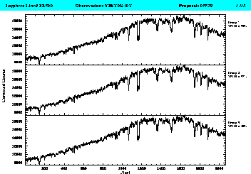
Output Data Products: IMAGE spectra
Image mode spectra are identified by an OPMODE value of IMAGE and a GRNDMODE value of IMAGE and a FGWA_ID of any spectral element except MIRROR. Normally, NXSTEPS=4 and OVERSCAN=5 were used to produce groups of 2064 pixels, but the full range of commandable values was allowed.
Usually one output group exists in the output data products for each raster spectrum line (YPOS) in the image. If more than one readout occurred (rare, but it could happen), then YSTEPS x NREAD groups exist in the data files. Each set of YSTEPS groups were accumulated in the same fashion as ACCUM mode measures, so that the last set of YSTEPS groups contains the accumulated spectra.
IMAGE mode spectra are not routinely flux calibrated by the pipeline because the x-position mapping to wavelengths is calibrated only for the aperture center Y-base. Therefore, the .c1* files are identical to the .c5* files (i.e. count rates corrected for everything but sensitivity).
Analysis: IMAGE spectra
The special FOS STSDAS routine yfluxcal can be used to flux calibrate IMAGE spectra on the assumption that the aperture-center wavelength calibration is applicable to the actual Y-base employed. This is a suitable assumption for virtually all calibration program IMAGE mode spectra.
.
[Top] [Prev] [Next] [Bottom]
1
Further details concerning polarimetry datasets and their calibration procedures can be obtained from within IRAF by typing "help spec_polar opt=sys".
2
See FOS ISR 078.
stevens@stsci.edu
Copyright © 1997, Association of Universities for Research in Astronomy. All rights
reserved.
Last updated: 01/14/98 14:29:35